Dreambooker

1. Background

There’re three ways to plot Polar satellite swaths data: pcolor, pcolormesh and imshow

I don’t recommend contourf because I want to keep the original data without interpolation.

The User Guide of matplotlib illustrates the differences between them in detail.

Here, I’ll show you the effects by some simple examples .

2. Definitions

pcolormesh

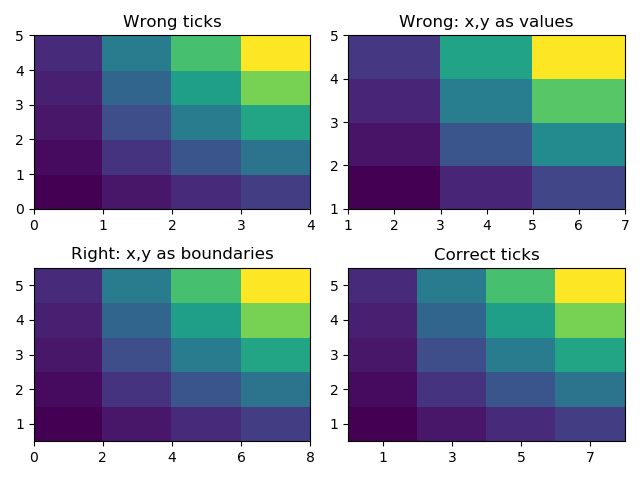
The definition of pcolormesh is plotting the C values with X,Y corners:

(X[i+1, j], Y[i+1, j])          (X[i+1, j+1], Y[i+1, j+1])
                      +--------+
                      | C[i,j] |
                      +--------+
    (X[i, j], Y[i, j])          (X[i, j+1], Y[i, j+1])

The figure below could help us understand that …

import pylab as pl
import matplotlib.pyplot as plt
import numpy as np

# values x and y give values at z
xmin = 1; xmax = 8; dx = 2
ymin = 1; ymax = 6; dy = 1
x,y = np.meshgrid(np.arange(xmin,xmax,dx),np.arange(ymin,ymax,dy))
z = x*y

# transform x and y to boundaries of x and y
x2,y2 = np.meshgrid(np.arange(xmin,xmax+dx,dx)-dx/2.,np.arange(ymin,ymax+dy,dy)-dy/2.)

fig, ((ax1, ax2), (ax3, ax4)) = plt.subplots(2, 2)
# pcolormesh without x and y just uses indexing as labels
ax1.pcolormesh(z)
ax1.set_title("Wrong ticks")

# pcolormesh with x and y values gives a wrong plot, x and y are treated as boundaries
ax2.set_title("Wrong: x,y as values")
ax2.pcolormesh(x,y,z)

ax3.set_title("Right: x,y as boundaries")
ax3.pcolormesh(x2,y2,z)
ax3.axis([x2.min(),x2.max(),y2.min(),y2.max()])

# using the boundaries gives correct plot
ax4.set_title("Correct ticks")
ax4.pcolormesh(x2,y2,z)
ax4.axis([x2.min(),x2.max(),y2.min(),y2.max()])
ax4.set_xticks(np.arange(xmin,xmax,dx))
ax4.set_yticks(np.arange(ymin,ymax,dy))

plt.tight_layout()
plt.show()

pcolor

Both methods are used to create a pseudocolor plot of a 2-D array using quadrilaterals.

The main difference lies in the created object and internal data handling: While pcolor returns a PolyCollection, pcolormesh returns a QuadMesh. The latter is more specialized for the given purpose and thus is faster. It should almost always be preferred.

There is also a slight difference in the handling of masked arrays. Both pcolor and pcolormesh support masked arrays for C. However, only pcolor supports masked arrays for X and Y. The reason lies in the internal handling of the masked values. pcolor leaves out the respective polygons from the PolyCollection. pcolormesh sets the facecolor of the masked elements to transparent. You can see the difference when using edgecolors. While all edges are drawn irrespective of masking in a QuadMesh, the edge between two adjacent masked quadrilaterals in pcolor is not drawn as the corresponding polygons do not exist in the PolyCollection.

Another difference is the support of Gouraud shading in pcolormesh, which is not available with pcolor.

imshow

If we use imshow to plot Swath data, we need to set extent and origin in the function.

extent : scalars (left, right, bottom, top), optional

The bounding box in data coordinates that the image will fill. The image is stretched individually along x and y to fill the box.

The default extent is determined by the following conditions. Pixels have unit size in data coordinates. Their centers are on integer coordinates, and their center coordinates range from 0 to columns-1 horizontally and from 0 to rows-1 vertically.

Note that the direction of the vertical axis and thus the default values for top and bottom depend on origin:

• For origin == 'upper' the default is (-0.5, numcols-0.5, numrows-0.5, -0.5).
• For origin == 'lower' the default is (-0.5, numcols-0.5, -0.5, numrows-0.5).

3. Comparison

Because pcolor and pcolromesh is similar, I will compare pcolormesh with imshow.

For imshow method, we need to use Pyresample to get the monotonous coordinates X and Y for extent.

I checked several tutorials online and find that they always use the center lons and lats as X and Y in pcolormesh.

That’s absolutely wrong !!! (If we care about the true values)

I choose one specific TROPOMI data which has an obvious region of low value.

Here’s the result with lcc projectoin:

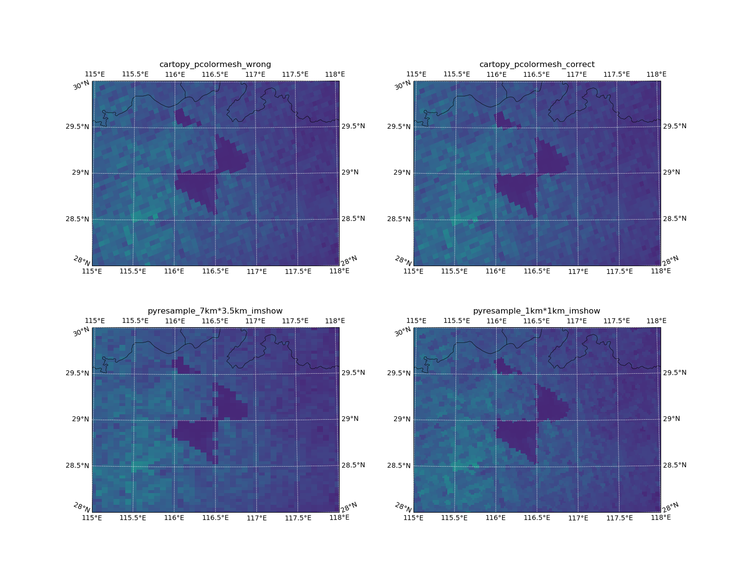
The difference between pcolormesh based on lons/lats centers and lons/lats bounds is half pixel.

It looks fine for TROPOMI if you just want check the overall distribution.

The resolution of TROPOMI is 7 km * 3.5 km (2018 – 2019/08/06) and 5.6 km * 3.5 km (2019/08/06 – now)

But, when you use this method to plot OMI data, that could result in big difference because of the lower resolution (24 km * 13 km).

BTW, if the resampling resolution is high enough, the result is almost as same as the “true” one.

4. Code

I use Satpy to read the TROPOMI data and cartopy to plot NO2 Vertical Column Densities (VCDs) on the map.

import sys
import os, glob
import numpy as np
import cartopy.crs as ccrs
from satpy.scene import Scene
import matplotlib.pyplot as plt
import cartopy.crs as ccrs
from pyresample.geometry import DynamicAreaDefinition

# My own modules
#   You can check it on the GitHub:
#   https://github.com/zxdawn/pyXZ
sys.path.append('../../XZ_maps/')
from xin_cartopy import add_grid, load_province, load_city

date = '20200219'
data_dir = '../data/tropomi/WH/'
file_pattern = '*{}*'.format(date)
filenames = glob.glob(data_dir + file_pattern)

def add_province(ax, provinces,
              west, east,
              south, north,
              lon_d, lat_d):
    ax.add_feature(provinces, edgecolor='k', linewidth=.3)
    add_grid(ax, ccrs.PlateCarree(),
              west, east,
              south, north,
              lon_d, lat_d,
              xlabel_size=10, ylabel_size=10,
              grid_color='whitesmoke')

def prepare_geo(latb, lonb, selection="both"):
    # Copy from PyCAMA:
    #    https://dev.knmi.nl/projects/pycama
    if latb.shape[0] == 1:
        dest_shape = (latb.shape[1]+1, latb.shape[2]+1)
    else:
        dest_shape = (latb.shape[0]+1, latb.shape[1]+1)

    dest_lat = np.zeros(dest_shape, dtype=np.float64)
    dest_lon = np.zeros(dest_shape, dtype=np.float64)

    if latb.shape[0] == 1:
        dest_lat[0:-1, 0:-1] = latb[0, :, :, 0]
        dest_lon[0:-1, 0:-1] = lonb[0, :, :, 0]
        dest_lat[-1, 0:-1] = latb[0, -1, :, 3]
        dest_lon[-1, 0:-1] = lonb[0, -1, :, 3]
        dest_lat[0:-1, -1] = latb[0, :, -1, 1]
        dest_lon[0:-1, -1] = lonb[0, :, -1, 1]
        dest_lat[-1, -1] = latb[0, -1, -1, 2]
        dest_lon[-1, -1] = lonb[0, -1, -1, 2]
    else:
        dest_lat[0:-1, 0:-1] = latb[:, :, 0]
        dest_lon[0:-1, 0:-1] = lonb[:, :, 0]
        dest_lat[-1, 0:-1] = latb[-1, :, 3]
        dest_lon[-1, 0:-1] = lonb[-1, :, 3]
        dest_lat[0:-1, -1] = latb[:, -1, 1]
        dest_lon[0:-1, -1] = lonb[:, -1, 1]
        dest_lat[-1, -1] = latb[-1, -1, 2]
        dest_lon[-1, -1] = lonb[-1, -1, 2]

    boolarray = np.logical_or((dest_lon[0:-1, 0:-1]*dest_lon[1:, 0:-1]) < -100.0,
                              (dest_lon[0:-1, 0:-1]*dest_lon[0:-1, 1:]) < -100.0)

    if selection == "ascending":
        boolarray = np.logical_or(boolarray, dest_lat[0:-1, 0:-1] > dest_lat[1:, 0:-1])
    elif selection == "descending":
        boolarray = np.logical_or(boolarray, dest_lat[0:-1, 0:-1] < dest_lat[1:, 0:-1])
    else: # "both"
        pass

    dest_lon[0:-1, 0:-1] = np.where(boolarray, 2e20, dest_lon[0:-1, 0:-1])

    return dest_lat, dest_lon

# ---------------- read data ---------------- #
scn = Scene(filenames, reader='tropomi_l2')
scn.load(['nitrogendioxide_tropospheric_column', 'qa_value', 
        'longitude', 'latitude', 'latitude_bounds', 'longitude_bounds'])

attrs = scn['nitrogendioxide_tropospheric_column'].attrs
# convert units
scn['VCD'] = 6.02214*1e4*scn['nitrogendioxide_tropospheric_column']
scn['VCD'].attrs = attrs
scn['VCD'].attrs['units'] = r'10$^{15}$ molec. /cm$^2$'

latb, lonb = prepare_geo(scn['latitude_bounds'], scn['longitude_bounds'], selection='both')
# ---------------- define map projection and lim ---------------- #
projection = {'proj': 'lcc', 'lat_0': 28.73997, 'lon_0': 116.3502, \
            'lat_1': 30, 'lat_2': 60, 'units': 'km'}

west = 115; east = 118
north = 30; south = 28
lon_d = 0.5; lat_d = 0.5

# ---------------- resample ---------------- #
low_res  = DynamicAreaDefinition('low_res', 'A low resolution area', projection, resolution = (7, 3.5))
scn_low  = scn.resample(low_res, radius_of_influence=10000)
crs_low  = scn_low['VCD'].attrs['area'].to_cartopy_crs()

high_res = DynamicAreaDefinition('high_res', 'A high resolution area', projection, resolution = (2, 2))
scn_high = scn.resample(high_res, radius_of_influence=10000)
crs_high = scn_high['VCD'].attrs['area'].to_cartopy_crs()

# ---------------- PLOT ---------------- #
fig = plt.figure(figsize=[15, 12])
provinces = load_province(ccrs.PlateCarree())
projection = crs_low

# ---------------- pcolormesh with cartopy ---------------- #
# -------- wrong pcolormesh -------- #
ax1 = plt.subplot(2, 2, 1, projection=projection)
add_province(ax1, provinces,
              west, east,
              south, north,
              lon_d, lat_d)

im = ax1.pcolormesh(scn['longitude'], scn['latitude'], scn['VCD'], transform=ccrs.PlateCarree())
ax1.set_title('cartopy_pcolormesh_wrong')

# -------- correct pcolormesh -------- #
ax2 = plt.subplot(2, 2, 2, projection=projection)
add_province(ax2, provinces,
              west, east,
              south, north,
              lon_d, lat_d)

im = ax2.pcolormesh(lonb, latb, scn['VCD'], transform=ccrs.PlateCarree())
ax2.set_title('cartopy_pcolormesh_correct')

# ---------------- imshow with pyresample ---------------- #
# --- imshow with pyresample (low resolution) --- #
ax3 = plt.subplot(2, 2, 3, projection=projection)
add_province(ax3, provinces,
              west, east,
              south, north,
              lon_d, lat_d)

ax3.imshow(scn_low['VCD'], transform=projection, extent=projection.bounds,
        origin='upper',interpolation='none')
ax3.set_title('pyresample_7km*3.5km_imshow')

# --- imshow with pyresample (high resolution) --- #
ax4 = plt.subplot(2, 2, 4, projection=projection)
add_province(ax4, provinces,
              west, east,
              south, north,
              lon_d, lat_d)

ax4.imshow(scn_high['VCD'], transform=crs_high, extent=crs_high.bounds,
        origin='upper',interpolation='none')
ax4.set_title('pyresample_1km*1km_imshow')

# ---- save fig ---- #
plt.subplots_adjust(wspace=0.3)
plt.tight_layout()
plt.show()

5. Conclusion

Overall, pcolormesh is the best tool to show the original/true data (if the lons and lats bounds are used).

But, if you want to compare Swath data with other sources like ground observations, other satellites data and model results, using pyresample with imshow or pcolormesh is the good option!

Version control